2 In the beginning…

2.1 Install and Use of R Studio

2.1.1 R and R Studio installed on a computer

Most users install R and R Studio on their computer. See Section 2.1.2 if you prefer not to install these or are in a position where you cannot install these (e.g. using a company computer).

Install The R Project for Statistical Analysis.
Install the free version of RStudio Desktop.

There are many online tutorials if you need help with the installation process.

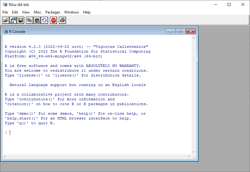
Once R and R Studio are installed, avoid RGui, which is what opens when you run R (Figure 2.1 and Figure 2.2). You can write R code with RGui, but it is much harder to use than R Studio.

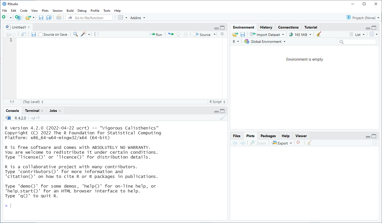
Instead, always run RStudio (Figure 2.3 and Figure 2.4)

You will write code in the Script window (Figure 2.15) and save the .R script file. Creating a new R script file and saving it is the start of this process. (Figure 2.5 through Figure 2.8)

Figure 2.7: You must select the directory and add the .R extension

2.1.2 R and R Studio in Posit Cloud

Posit Cloud has various subscription options, including a Free option that is limited to 25 hours per month and a Plus plan for $5 per month that is limited to 75 hours per month.

Once you have your Posit Cloud account, you can create a new project to launch R Studio in Posit Cloud (Figure 2.9 through Figure 2.12)

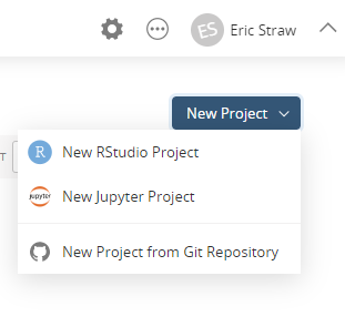
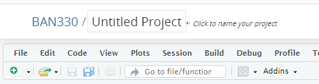
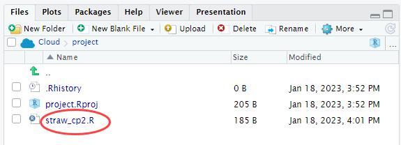
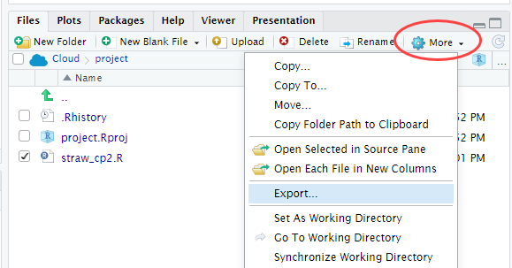
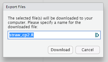
Figure 2.12: Posit adds the .R extension

You can download your R script file (Figure 2.13 and Figure 2.14) to save it locally or share it. The file downloads to your browser’s download directory.

Figure 2.13: Select the file > More > Export

2.1.3 R Studio layout both Installed and Posit Cloud

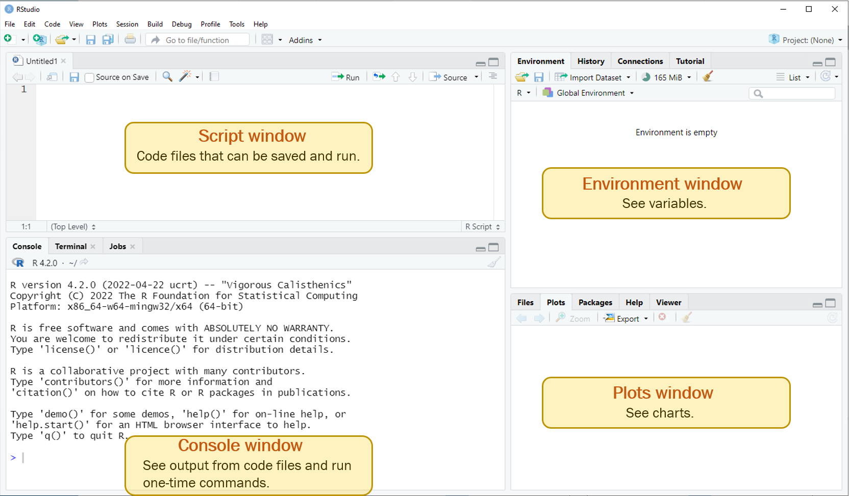
2.2 Create and Use Objects

Object: An object is a bucket that holds values – aka variable

We use the assignment operator <- to assign values to objects. The following line of code can be read as “object x gets 5” or “variable x gets 5” or “x gets 5”.

x <- 5

x is a wonderful variable name in mathematics. It is a terrible object name in programming. Use meaningful names. Separate words with the underscore character. Notice the comment in the next block of code using the # symbol. This comment shows how to read the line of code. You should include abundant comments in your code. Comments will save you much time in learning to program. Type the lines of code in the Script window. What happens when you press Enter at the end of the last line of code? Nothing!

# day_one gets 25
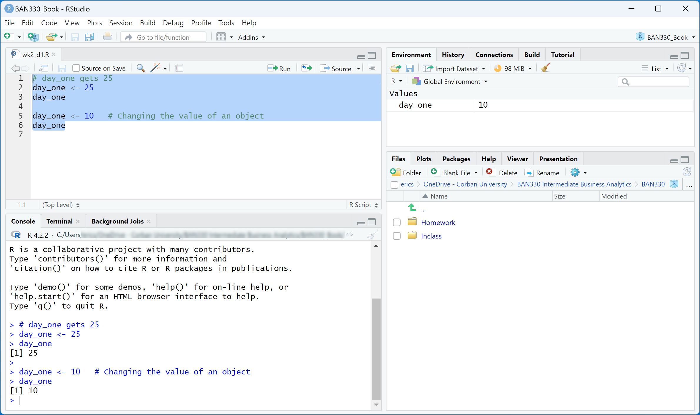
day_one <- 25

In Figure 2.16 the Run button runs the line where the cursor is located, or the lines selected by highlighting with left-mouse + drag, and the Source button runs the entire script. Run will generate output to the Console window. Source will not generate output to the Console window.

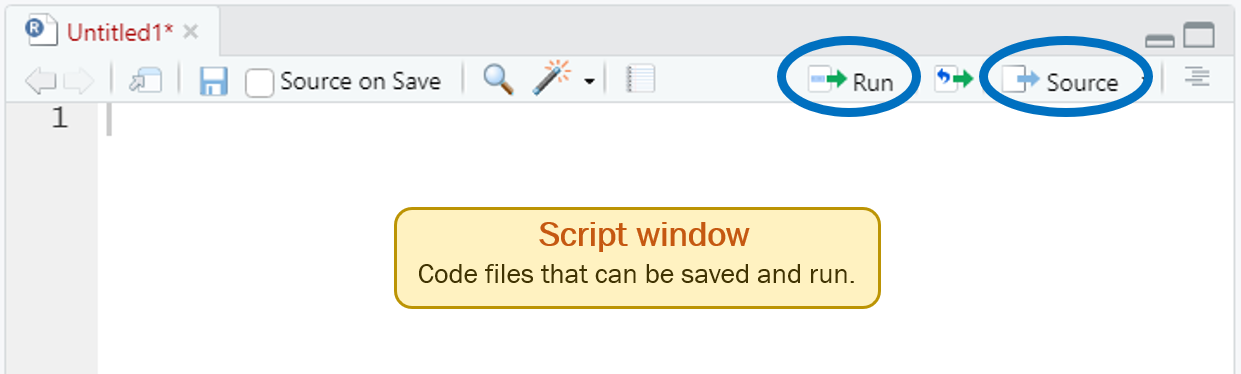
Run your code by using Source.

Print the object day_one to the Console window by typing the name of the object in the Script window as shown below. Place your cursor anywhere on this new line of code and run it by using Run.

# day_one gets 25
day_one <- 25
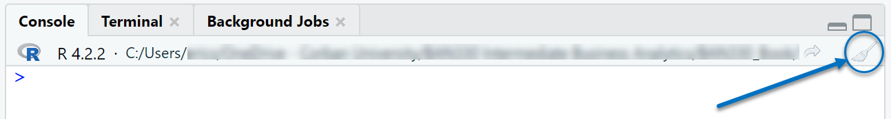
day_one

Clear the Console window with the broom icon on the right-hand side of the Console window. This icon is always faint and looks grayed-out, but it works. Alternatively, you can use the keyboard shortcut CTRL+L to clear the Console window.

Figure 2.17: Broom to clear the Console window

Now run the whole script by using Source. Does the output show in the Console window?

Now run the whole script by highlighting the code and using Run. Does the output show in the Console window?

Run will generate output to the Console window. Source will not generate output to the Console window.

Now type day_one in the Console window at the > prompt and press the Enter key. What happens?

You can enter and immediately run code in the Console window. However, you should avoid doing this because the Console window code is not saved. Instead, always enter your code in a script and save your script file. This guidance only applies to beginning programmers. As you learn to code you will learn when you should use the Console window.

What happens when you add the following code to the Script window and run it?

The assignment operator <- always stores the value in the object (the bucket), which causes the previous contents of the object to be lost.

# day_one gets 25
day_one <- 25
day_one

day_one <- 10   # Changing the value of an object
day_one

2.3 Scripts

File management and version management are critical for successful coding. Here is a simple process to get you started.

Create a folder for your R projects
Create sub folders for each project
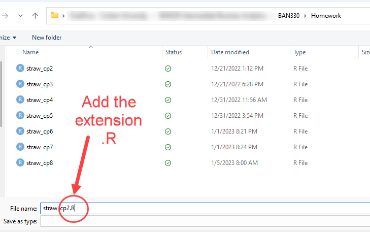
Save your script file to your project sub folder – remember to add the .R extension
Close the script tab, then close R
Navigate to your project sub folder and open your R script file, R should open
Run the entire script using Run – Remember, you must first highlight all the lines of code
Notice the Environment window. Your RStudio should look like Figure 2.18 if you are reproducing the code in this demonstration
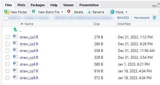
You can navigate to your project sub folder in the Files window of RStudio

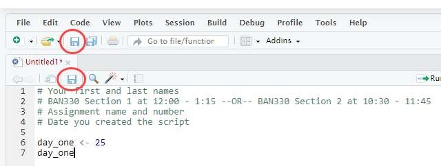
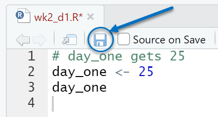
Delete the last two lines of code from your script. Notice the name of your script is red. This means that changes have been made but not yet saved. Save your script now by using the disk icon right below the name of the script.

2.4 Operators

Resource: W3Schools operators

Operator: An operator is a symbol that performs a specific task (e.g. the + symbol performs addition).

Enter the following code and notice what happens to the object day_one with each assignment.

# day_one gets 25
day_one <- 25
day_one

day_one <- day_one + 5
day_one

second_number <- 10
day_one <- day_one + second_number
day_one

day_one <- day_one / 4
day_one

day_one <- day_one * 2.5
day_one

day_one <- (day_one - 5) / 4
day_one

day_one <- 3
day_one <- day_one ^ 2
day_one

You will use many more operators as you develop your programming skills.

2.5 Functions

Resource: Huynh chapter 3, section 3.3, subsections 3.3.1 through 3.3.8

Functions in R are like functions in Excel. The pattern is: function_name(argument_1, argument_2, ... argument_N).

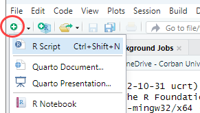
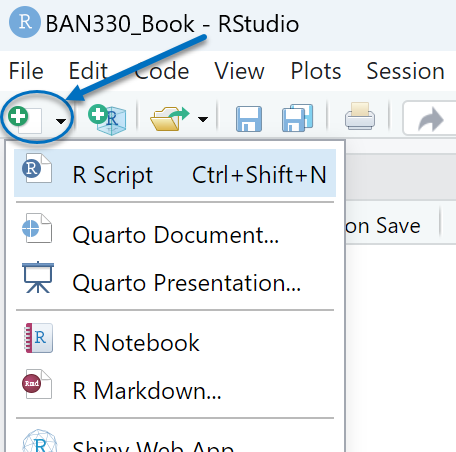
Create a new script tab by selecting the green plus icon shown in Figure 2.20 then select R Script. You can also use the keyboard shortcut.

Best practice: Clear R Studio when switching to a new project and often when troubleshooting.

Clear the Console window by using the broom icon shown in Figure 2.17 or with the keyboard shortcut CTRL+L.
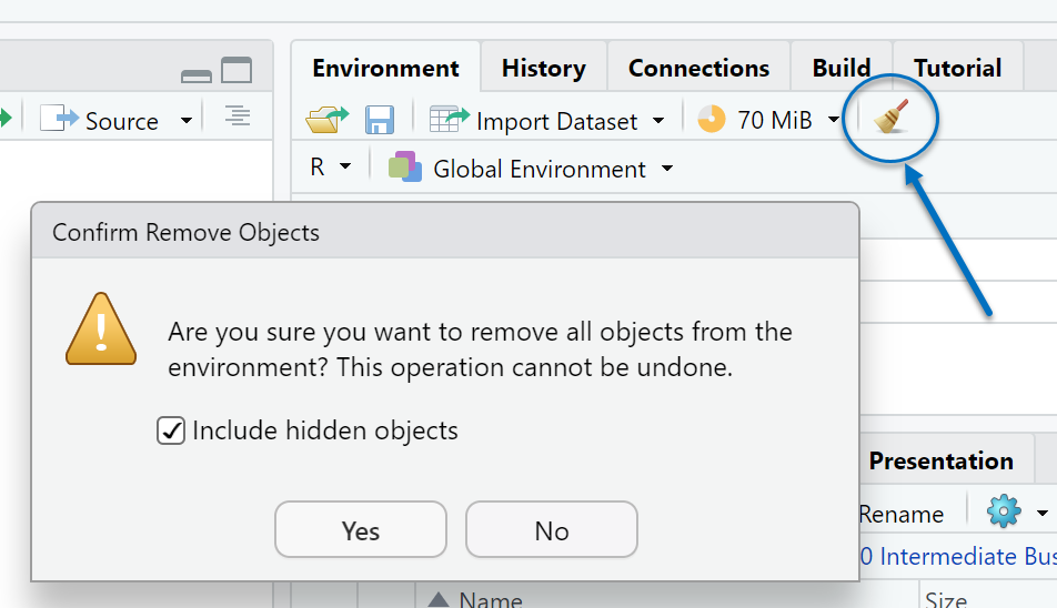
Clear the Environment window by using the broom icon shown in Figure 2.21. A dialogue box will appear. Check the “Include hidden objects” box and then select Yes. This clears the R environment of all objects.

Enter the following code in your new script tab and run it. What can you learn about functions in R from the results? Remember, to be abel to see the results in the Console window you must either use Run on each line of code or highlight all the code and use Run.

# Use the round() function to round the value stored in the object first_number
first_number <- 8.4395
round(first_number)
first_number
first_number <- round(first_number)
first_number

R functions process and display results but do not store results. You must use the assignment operator if you want to store the results of an R function.

Try this next set of code to see how the second argument in the round() function works.

# Use the `digits` argument in the round() function
first_number <- 8.4395
second_number <- round(first_number, digits = 2)
second_number

first_number <- 264751.89
second_number <- round(first_number, digits = -3)
second_number

Functions can be embedded inside other functions. Run the following code and evaluate the results. Notice the sequence of settings inside the quotation marks within the format() function. These settings tell the format() function how to format the date and time for display. This R-blogger.com article has a full list of the possible settings and much more about working with the system time. Search for %A to find the table of possible settings in the linked article.

# Display the system day and time
# Format the output of the system day and time with the format() function
Sys.time()
format(Sys.time(), "%A %b %d, %Y at %R")

Remember, functions process and display results but do not store the results. If you want to store the results of a function you must assign the results to an object as shown below.

# Assign the formatted date and time to an object
homework_done <- format(Sys.time(), "%A %b %d, %Y at %R")

2.6 Write Code for People

Resource: Wickham chapters 1, 2, and 3

Writing code for people is possibly the most important thing you can learn as a new programmer. We have focused on the following guidelines for writing code for people.

Object names: Use descriptive names with the underscore character between words. Object names should be descriptive, but not too long. Length is a matter of preference.
File names: Similar to object names.
Spacing: Include a single space after each element in a line of code except parentheses. The following line of code demonstrates proper spacing: homework_done <- format(Sys.time(), "%A %b %d, %Y at %R")
Comments: Contrary to Wickham, chapter 3, section 3.4, you should use comments to explain the how, what, and why. Your future self will thank you for this practice. Comment liberally! As your coding becomes more complex you should include links to web resources that helped you with your code as well as explain what you were thinking and why you chose to solve the problem the way you did.

2.7 Debug

Coding is learned through practice, just like driving a car or swinging a bat. Debugging (aka troubleshooting) is an integral part of coding and can be frustrating to learn. To program well, you must choose to be extremely careful and pay attention to all details. The computer will only do exactly what you tell it to do. Debugging requires extreme determination. Stick with it. You can find a solution to every problem.

Programming allows for rapid prototyping. Unlike building a house, programming allows you to build something (i.e. attempt to run code) and tear it down (i.e. comment it out or delete it) if it does not work. Keep pressing forward. You can find a solution to every problem.

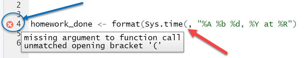
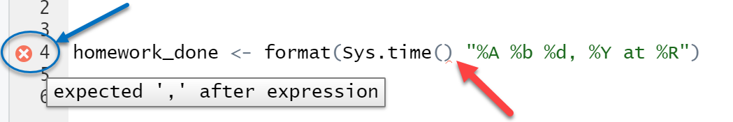
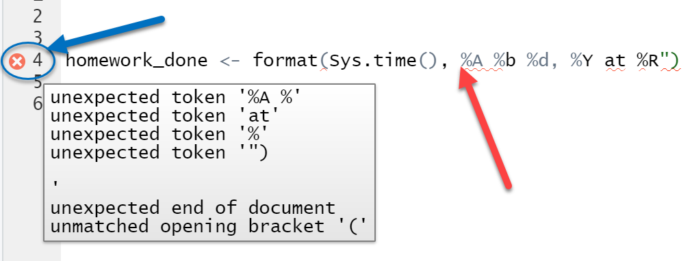
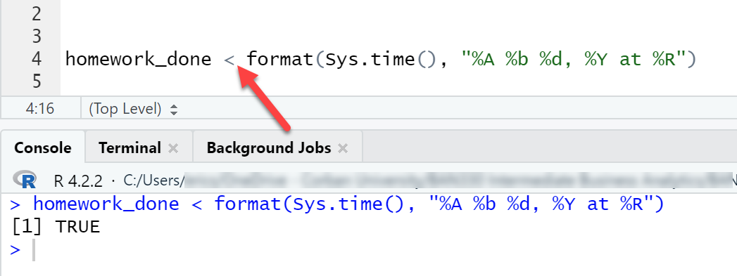
Figure 2.22 illustrates several programming errors and their results. You can hover your mouse over the red-X when it appears next to the line of code with the problem. These error messages are sometimes helpful, but not always. Notice the Missing Quotation problem in (c). The error message does not identify the real problem. Notice the Incomplete Assignment Operator problem in (d). No error message is generated and the line of code runs successfully. However, the results are not what we expect with the assignment operator. The < in (d) is a less than operator, which results in the value TRUE being returned.

You will have to debug your code. No one writes perfect code on the first attempt. Extreme attention to detail and persistence are required to find errors when you fail to correctly type code.

Figure 2.22: Debugging Examples

2.8 Object Types

Resource: Rodrigues chapter 2, section 2.1 through 2.7

Object: An object is a bucket that holds values – aka variable

Different kinds of objects, like different buckets, have characteristics that define what the object can be used for. We do not haul milk in a cement truck. Nor do we put drinking water in a trash can. Learning to recognize and use the correct bucket is important.

Vector: A vector is the basic storage unit in R that can hold only one data type. Comparable to a single cell and multiple cells in Excel.

We will focus on four vector data types: character, double, integer, and logical. A vector can contain only one data type. A table of all possible data types can be found in R Language Definition chapter 2.

Character type

# This character type, like a single cell in Excel
# first_char is a vector
first_char <- "BAN330"
typeof(first_char)
is.character(first_char)
length(first_char)
first_char

# This character type, like multiple cells in Excel 
# The combine function -- c() -- is used to combine the individual values
# second_char is a vector
second_char <- c("BAN330", "BUS335", "BUS403", "BUS473")
typeof(second_char)
is.character(second_char)
length(second_char)
second_char
second_char[1]
second_char[2]
second_char[3]
second_char[4]

# Replace an element
second_char
second_char[2] <- "BAN320"
second_char

# Add a new element
second_char
second_char[5] <- "BUS335"
second_char[6] <- first_char
second_char

# Paste character types together
word_1 <- "Data"
word_2 <- "digital economy"
my_sentence <- paste(word_1, "is the life-blood of the", word_2)
my_sentence

Double type

# This double type, like a single cell in Excel
# first_number is a vector
first_number <- 25
typeof(first_number)
length(first_number)
is.character(first_number)
is.double(first_number)
first_number

# This double type, like multiple cells in Excel 
# The combine function -- c() -- is used to combine the individual values
# second_number is a vector
second_number <- c(10, 15, 20)
typeof(second_number)
is.character(second_number)
is.double(second_number)
length(second_number)
second_number
second_number[1]
second_number[2]
second_number[3]

# Replace an element
second_number
second_number[1] <- 5
second_number

# Add a new element
second_number
second_number[4] <- first_number
second_number[5] <- 30
second_number

# Math with double types
answer_1 <- first_number * 2
answer_1
answer_2 <- second_number[3] / 2
answer_2
answer_3 <- (first_number - second_number[2]) ^ 2
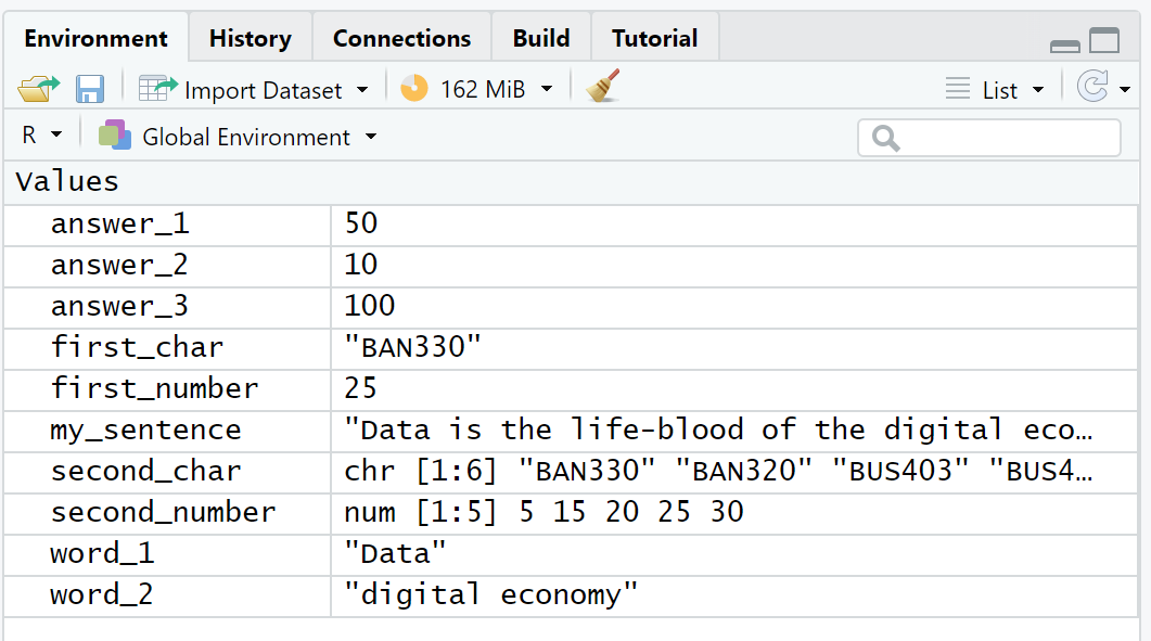
answer_3

You can view objects without printing them to the Console window by looking at the Environment window. Notice the character types are in quotation marks. Also notice the format of the vectors with multiple values. From here on out the examples will not include the line of code to print the value to the Console window. You can look at the Environment window and/or add the line of code as desired.

Integer Type

The Integer type functions like the Double type. However, the Integer type can only hold integers (i.e. no fractions).

# This integer type, like a single cell in Excel
# first_integer is a vector
first_integer <- 5L
typeof(first_integer)
length(first_integer)
is.character(first_integer)
is.double(first_integer)
is.integer(first_integer)

second_integer <- 20L

# R will often convert the result into a double type
answer_4 <- first_integer + second_integer
typeof(answer_4)
answer_5 <- second_integer / first_integer
typeof(answer_5)
answer_6 <- second_integer / 3
typeof(answer_6)

# Two methods of forcing division to return an integer (i.e. discard fractions), 
# but it still returns a double type
answer_7 <- second_integer %/% 3
typeof(answer_7)
answer_8 <- floor(second_integer / 3)
typeof(answer_8)

# Use the as.integer() function to force the Integer type
answer_9 <- as.integer(floor(second_integer / 3))
typeof(answer_9)

Logical Type

A Logical type can only have one of two values: Either TRUE or FALSE.

# This line of code will return FALSE because 25 is NOT less than 15
# Read the line as, "Is 25 less than 15?"
25 < 15

# This Logical type, like a single cell in Excel
# first_logical and second_logical are each vectors
first_logical <- 25 < 15
typeof(first_logical)

second_logical <- 25 > 15
typeof(second_logical)

# These Logical type, like multiple cells in Excel 
# The combine function -- c() -- is used to combine the individual values
# third_logical and fourth_logical are each vectors
third_logical <- c(TRUE, TRUE, FALSE)
typeof(third_logical)
fourth_logical <- c(TRUE, TRUE)
typeof(fourth_logical)

# replace and add elements to a Logical type
fourth_logical[1] <- FALSE
fourth_logical[3] <- FALSE

# Compare elements in a Logical type using the AND operator &, 
# which returns TRUE only if both values are TRUE
# This operator compares third_logical[1] AND fourth_logical[1], 
# then third_logical[2] AND fourth_logical[2], etc.
answer_10 <- third_logical & fourth_logical

List: A storage unit in R that can hold multiple data types.

# Example of a list holding all the above data types
# Note the use of the `list()` function instead of the combine function
list_1 <- list("one", "two", 3, 4, 5L, 6L, TRUE, FALSE)
typeof(list_1)       # Returns "list"

# Elements in a list can be accessed and changed just like elements in a vector
list_1[2] 
list_1[2] <- "We changed this value"

# Elements can be added to a list just like a vector
list_1[9] <- "Added element"
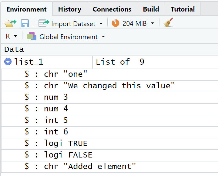
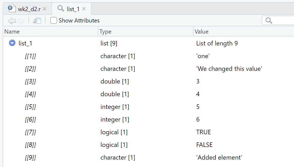
list_1

Expanding the list_1 object in the Environment window by left-clicking on the expand symbol (blue dot with white triangle) will show the types of all the elements in the list as shown in Figure 2.24. Viewing list_1 by left-clicking the object name in the Environment window or running the function view(list_1) will show the types and other details as shown in Figure 2.25.

Figure 2.24: A list object in the Environment window

2.9 Change Data Types

Resource: Rodrigues chapter 2, section 2.1 through 2.7

Intentionally changing a data type is done through the as. functions. Each of the data types covered in this chapter have an as. function.

# Convert an Integer type to a Character type
first_integer <- 25L
typeof(first_integer)

first_char <- as.character(first_integer)
typeof(first_char)

# Convert a Character type to a Double type
first_double <- as.double(first_char)
typeof(first_double)

The change of a data type will fail if the value is not compatible with the new data type. Notice the warning message in the Console window and the value of second_double object when you run the following code.

# The value in the Character type *second_char* is not compatible with the Double type
second_char <- "This will not work"
second_double <- as.double(second_char)