6 Binary Logistic Regression
6.1 Introduction to Logistic Regression
There are several forms of logistic regression:
Multinomial logistic regression (a.k.a nominal logistic regression) is based on a nominal y variable with more than two categories. Nominal variables are categorical variables (a.k.a qualitative variables) that are different in name only (i.e. there is no inherent order in the categories). For example, eye color represented with category names such as blue, brown, green or represented with category names such as 0, 1, and 2. See Hua, Choi, and Shi (2021) chapter 11 for an example.
Binary logistic regression (the topic of this chapter) is based on a binary y variable. Binary variables are categorical variables (a.k.a qualitative variables) that are nominal variables represented with only two categories. For example, the answer to a survey question represented with category names such as yes and no or represented with category names such as 0 and 1. See Hua, Choi, and Shi (2021) chapter 10 for an example.
Ordinal logistic regression is based on an ordinal y variable. Ordinal variables are categorical variables (a.k.a qualitative variables) that are different in name and order. For example, quality rating represented with category names such as good, better, best, or represented with category names such as 0, 1, and 2. See Hua, Choi, and Shi (2021) chapter 12 for an example.
Logistic regression models do not estimate the y variable like linear regression models. Instead, logistic regression models estimate the probability of the y variable being a specific category. For example, in binary logistic regression with category names 0 and 1, the model estimates the probability that y is in the category 1.
6.1.1 Logistic regression equation
The final form of the logistic regression equation (Equation 6.1) differs from the linear regression equation on the left side of the equation. The right side of the equation continues to have x variables and corresponding coefficients (a.k.a parameters) represented by β0, β1, β2, β3, …, βn. However, β0 is not the y-intercept.
\[logit(p) = \beta_{0} + \beta_{1}x_{1} + \beta_{2}x_{2} + \beta_{3}x_{3} + ... + \beta_{n}x_{n} \tag{6.1}\]
6.1.1.1 Left side of the equation
We begin with the concepts of odds (Equation 6.2) and probability (Equation 6.3). For example, if the probability of an event occurring is 80%, then the odds of the event occurring are 4:1 because \(\frac{80}{(1-80)} = 4\). If the odds of an event occurring are 4:1 then the probability of the event occurring is 80% because \(\frac{4}{(1+4)} = 0.80\).
\[odds = \frac{p}{1-p} \tag{6.2}\]
\[p = \frac{odds}{1+odds} \tag{6.3}\]
Logistic regression modeling relies on natural logarithm, which means the base is \(e\) (a.k.a Euler’s number). The value of \(e\), much like \(π\), is a mathematical constant with special properties (Aghaeiboorkheili and Kawagle (2022)). The value of \(e\) to 15 decimal places is 2.718281828459045. Equation 6.4 and Equation 6.5 illustrate the meaning of a logarithm, specifically a natural logarithm because the base is \(e\).
\[log_{e}(a) = b \tag{6.4}\] \[e^b = a \tag{6.5}\]
The left side of the logistic regression equation can be represented in one of the equivalent forms in Equation 6.6 where \(odds\) are the odds of \(y = 1\) and \(p\) is the probability of \(y = 1\). The final form, \(logit(p)\) is the most common form used to represent the left side of the logistic regression equation. The term logit refers to a logistic transformation of the odds.
\[log_{e}(odds) = log_{e}(\frac{p}{1-p}) = logit(p) \tag{6.6}\]
Thus, the logistic regression equation produces the logit of \(p\), which is the natural log of the odds of \(y = 1\). This value ranges from 0 to 1 and is interpreted as the probability that \(y = 1\). This probability is then rounded to create the categories \(y = 1\) or \(y = 0\). The rounding threshold depends on the application. The common practice of using 0.50 as the rounding threshold works for many situations.
6.1.1.2 Right side of the equation
The coefficients on the right side of the logistic regression equation are estimated using the maximum-likelihood method. The equations for maximum-likelihood estimation (MLE) are beyond the scope of this chapter. See STAT415 (n.d.) for details.
The coefficients (β1, …, βn ) are interpreted as follows (UCLA (n.d.a)).
For continuous \(x\) variables, a one-unit change in the \(x\) variable causes the \(logit(p)\) (i.e. natural log of the odds of \(y = 1\)) to change by the value of the coefficient of that \(x\) variable.
For binary categorical \(x\) variables, a value of \(x = 1\) causes the \(logit(p)\) (i.e. natural log of the odds of \(y = 1\)) to change by the value of the coefficient of that \(x\) variable because \(1 * β = β\). In contrast, a value of \(x = 0\) causes no change in the \(logit(p)\) because \(0 * β = 0\).
6.1.2 Logistic regression concept
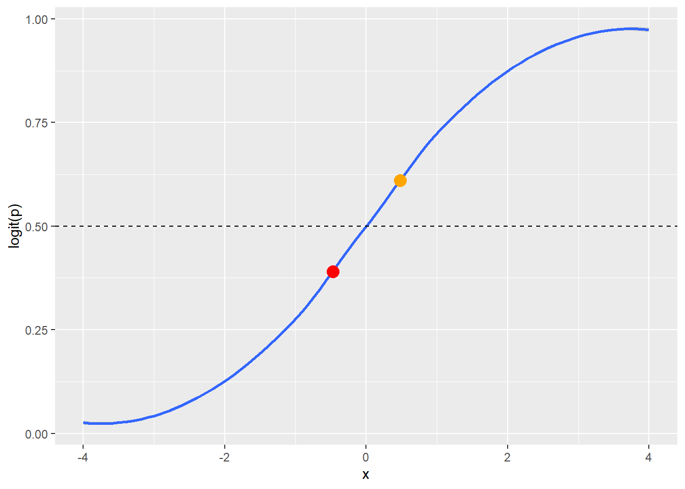
The \(logit(p)\) (i.e. natural log of the odds of \(y = 1\)) is always bounded between 0 and 1 and forms a sigmoidal shape (i.e. an s-curve, blue line in Figure 6.1). Values of the \(logit(p)\) fall on this line and are interpreted as \(y = 1\) or \(y = 0\) based on a rounding threshold. The rounding threshold depends on the application. The common practice of using 0.50 as the rounding threshold works for many situations. The 0.50 rounding threshold (dashed line in Figure 6.1) would convert the orange dot into \(y = 1\) and the red dot into \(y = 0\) (Figure 6.1).
6.2 Binary Logistic Regression Assumptions
As with assumptions of linear regression model building (Section 5.2), explanations of the assumptions of logistic regression model building are all over the board. Quite surprisingly, none of the resources used in Section 5.2 (Freund and Wilson (2003), Groebner, Shannon, and Fry (2014), Jaggia et al. (2023), Shmueli et al. (2023), and Statistics by Jim) contain information about the assumptions of logistic regression. The assumptions of logistic regression belong to statisticians, not data analysts. I am not a statistician. I have gleaned the following assumptions from reconciling the explanations in Foley (2022, chap. 2, section 1), Hua, Choi, and Shi (2021, chap. 10, section 2), James et al. (2022, chap. 4, section 17), Leung (2021) with GitHub page, and Schreiber-Gregory and Bader (2018),
I am convinced that at least part of the problem with the disparity in descriptions is the use of the word assumptions. What do we mean by assumptions? We mean requirements of the model that should be checked, and if you do not check these requirements then you are assuming they are true.
A logistic regression model that violates one or more of these assumptions may still be useful for estimating \(y\) values.
Logistic regression model building requirements that should be checked or assumed.
Categorical \(y\) variable: The \(y\) variable must meet the form of logistic regression being performed (Section 6.1): Multinomial; binary; or ordinal. Logistic regression is not suited for calculating a continuous \(y\) variable.
Linearity with \(logit(p)\): There is a linear relationship between each continuous \(x\) variable as specified and the \(logit(p)\) (i.e. natural log of the odds of \(y = 1\)). The as specified refers to the form of the \(x\) variables (e.g. no transformation, raised to a power, inverse, log, etc.). This can be checked with scatter plots and the Box-Tidwell test (See Section 6.3.1 and Foley (2022) Assumptions).
Low multicolinearity: Multicolilnearity refers to a linear relationship between any of the x variables {x1, x2, x3, …, xn}. We want little to no multicolinearity among our x variables because linear relationships between the x variables adversely impacts the accuracy of the coefficient calculations. Variance Inflation Factor (VIF) can be used to test for multicolinearity among the x variables. Pairwise scatter plots can be used to visually evaluate multicolinearity among the x variables.
Independent observations: The observations (i.e. rows of data) are not correlated with one another. Observations that are correlated will cause repeating patterns in the errors.
The following are not requirements that should be checked, but are important considerations.
- Linearity in coefficients: The equation is linear in the coefficients {β1, β2, β3, …, βn}, which means no coefficient is raised to a power (other than 1) and there is no multiplication or division of a coefficient by another coefficient. This means the form of Equation 6.1 is the only possible form of coefficients for a logistic regression equation. The functions used in R ensure this linearity of coefficients. This does not prevent the x variables {x1, x2, x3, …, xn} from being mathematically altered (e.g. raised to a power, inverse, log, etc.) to increase the estimation ability of the model.
6.3 Maximum Likelihood Estimation
The glm() function is used to run MLE logisitic regression. The first parameter of the glm() function is the variables to be used in the equation. Equation 6.7 illustrates the basic form of this parameter, which is used when there is no interaction in x variables. The ‘+’ sybmol in Equation 6.7 can be read as and.
\[y \sim {x}_{1} + {x}_{2} + {x}_{3} + ... + {x}_{n} \tag{6.7}\]
The second parameter of the glm() function is the family or type of model. We use binomial for binary logistic regression.
The example below includes variables named \(y\), \(x1\), and \(x2\). You can use your imagination to think about \(y\) as some yes or no variable which we are attempting to estimate based on two continuous \(x\) variables.
# Read in the fake data
fake_data <- read_csv("fake_logistic2.csv")

# Create the linear regression model
my_model <- glm(y ~ x1 + x2, family = "binomial", data = fake_data)
The results of glm() should be stored in an object, my_model in this example, and can be summarized with the summary() function.
# Output the summary report of the binary logistic regression model
summary(my_model)
Call:
glm(formula = y ~ x1 + x2, family = "binomial", data = fake_data)

Deviance Residuals:
    Min       1Q   Median       3Q      Max
-2.4965  -0.7282  -0.2097   0.6544   1.7820

Coefficients:
            Estimate Std. Error z value Pr(>|z|)
(Intercept) -11.8702     3.8872  -3.054 0.002261 **
x1            1.2952     0.3852   3.362 0.000773 ***
x2            0.9664     0.3711   2.604 0.009205 **
---
Signif. codes:  0 '***' 0.001 '**' 0.01 '*' 0.05 '.' 0.1 ' ' 1

(Dispersion parameter for binomial family taken to be 1)

    Null deviance: 68.029  on 49  degrees of freedom
Residual deviance: 42.226  on 47  degrees of freedom
AIC: 48.226

Number of Fisher Scoring iterations: 5
The summary output provides \(β_{0}\) (Figure 6.2, green box) and coefficients for the \(x\) variables (Figure 6.2, yellow box), which allows us to write the equation in Equation 6.8.
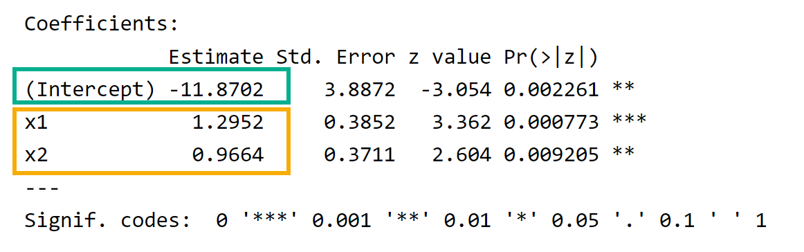
\[logit(p) = -11.87 + 1.30 * x_{1} + 0.97 * x_{2} \tag{6.8}\]
6.3.1 Checking linearity with \(logit(p)\)
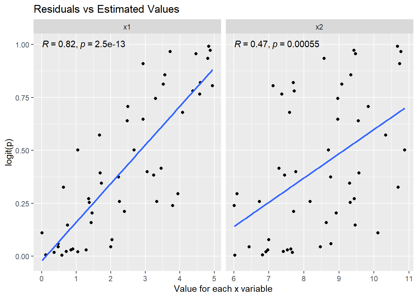
You may recall that one of the requirements that should be checked (Section 6.2) is the linearity of each \(x\) variable with the \(logit(p)\). This can be checked visually (Figure 6.3) and by using the Box-Tidwell test. See Foley (2022) Assumptions for details on running the Box-Tidwell test.
library(tidyr)   # for pivot_longer function
library(ggpubr)  # for stat_cor function to add Pearson correlation to the plot

# Prepare the data set for plotting the estimated y values against each x variable

# Copy the original data frame. I am always reluctant to change my original data frame
#   even though I know that I can simply read in the CSV file again to restore my
#   original data frame.
print_data <- fake_data

# Add the fitted values from the model
print_data$fitted <- my_model$fitted.values

# Pivot the x variables to columns
# Label the new column "x-variables"
# The value of teach x variable will be moved into a column named "value"
print_data <- print_data |>
  pivot_longer(c(x1, x2), names_to = "x_variables")

# View the prepared data frame
head(print_data)
# A tibble: 6 × 4
y fitted x_variables value
<dbl> <dbl> <chr> <dbl>
1 1 0.820 x1 4.59
2 1 0.820 x2 7.7
3 0 0.0304 x1 1.29
4 0 0.0304 x2 6.97
5 1 0.502 x1 2.68
6 1 0.502 x2 8.7 # Create a plot for each x variable
ggplot(data = print_data,
mapping = aes(x = value, y = fitted)) + # value is the data frame variable containing the values of each x variable
geom_point() +
facet_wrap(facets = vars(x_variables), scales = "free_x") + # Create side-by-side plots based on x variables
geom_smooth(method = "lm", formula = "y ~ x", se = FALSE) + # Add the linear model line
stat_cor(method = "pearson", label.y = 1) + # Add the Pearson correlation and p-value
labs(
title = "Residuals vs Estimated Values",
x = "Value for each x variable",
y = "logit(p)"
)
The visual approach in this section is adapted from Foley (2022) Assumptions.
I have added the Pearson correlation (Figure 6.3) for measuring the linear relationship between \(logit(p)\) and each \(x\) variable. The Pearson correlation for \(x1\) is strong (\(R = 0.82\)) and statistically significant (\(p < 0.05\)). The Pearson correlation for \(x2\) is moderate (\(R = 0.47\)) and statistically significant (\(p < 0.05\)). See Frost (n.d.) for details on interpreting Pearson correlation.
6.4 Model Performance Metrics
- Deviance Measures
-
The Null Deviance and Residual Deviance can be used to calculate chi-square (Equation 6.9) and the associated p-value {Equation 6.10} to evaluate the quality of the model.
\[\chi^2 = null \ deviance - residual \ deviance \tag{6.9}\]
\[p{-}value_{\chi^2} = df_{null \ deviance} - df_{residual \ deviance} \tag{6.10}\]
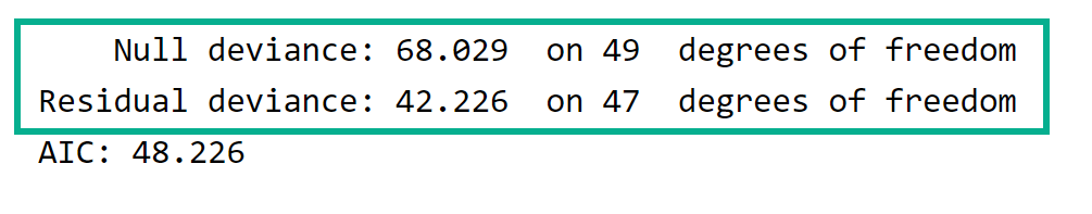
Here are the calculations for our example. These values can be calculated from results in the model and used to calculate the p-value of chi-square as shown in the code example.
\(\chi^2 = 68.029 - 42.226 = 25.803\)
\(p{-}value_{\chi^2} = 49 - 47 = 2\)
# calculate chi-square as null deviance - residual deviance
chi2 <- my_model$null.deviance - my_model$deviance

# Calculate chi-square degrees of freedom as df{null deviance} - df{residual deviance}
pv_chi2 <- my_model$df.null - my_model$df.residual

# Calculate the p-value for chi-square
pchisq(q=chi2, df=pv_chi2, lower.tail=FALSE)
[1] 2.494247e-06The p-value shown above is less than the chosen significant level of 0.05. Thus, the model is acceptable to use for estimating the \(y\) variable.
- Akaiki Information Criterion (AIC)
-
AIC is used to compare different models developed on the same data set. AIC is based on log-likelihood and includes a penalty for increasing the number of \(x\) variables. A lower AIC indicates a better model for that data set. AIC is not an absolute measure and cannot be used to evaluate a single model. It can only be used to compare two or more models developed on the same data set.
- Pseudo R-Square
-
Pseudo R-square is not shown in the
summary()output. However, Pseudo R-square is a model evaluation metric for logistic regression. There are many possible formulas for Pseudo R-square (UCLA (n.d.b)). Pseudo R-square is not like R-square for linear regression! (1) The range of Pseudo R-squared is not limited to 0-1, (2) Pseudo R-squared does not represent the amount of variation in the dependent variable that is explained by the independent variables. Pseudo R-square is used to compare different models developed on the same data set. A higher Pseudo R-square, calculated with the identical formula, indicates a better model for that data set. Pseudo R-square is not an absolute measure and cannot be used to evaluate a single model. It can only be used to compare two or more models developed on the same data set. - Confusion Matrix
-
The confusion matrix is not shown in the
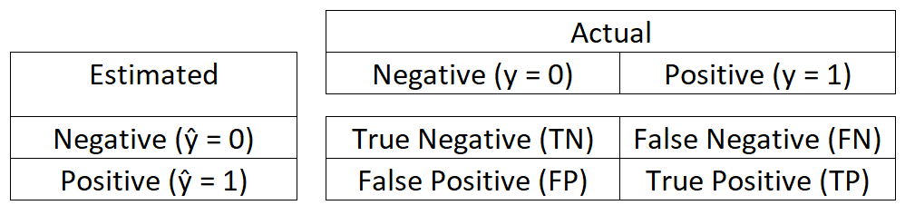
summary()output. It must be generated using a function. The confusion matrix produces the best performance metrics for logistic regression. Specifically, the Accuracy measurement. A confusion matrix compares the count of false negatives, true negatives, false positives, and true positives. These counts are calculated from comparing \(\hat{y}\) (estimated \(y\)) with the actual \(y\) for each observation.
True positive (\(TP\)) is when \(\hat{y} = y = 1\)
False positive (\(FP\)) is when \(\hat{y} = 1\) but \(y = 0\)
True negative (\(TN\)) is when \(\hat{y} = y = 0\)
False negative (\(FN\)) is when \(\hat{y} = 0\) but \(y = 1\)
The confusion matrix is displayed as a 2 x 2 matrix where the intersection of rows and columns hold the count of the true and false values described above.
library(caret)    # for the confusionMatrix() function

# Calculate the estimate for each observation based on rounding of the logit(p) for each observation
# The round() function uses the default threshold of 0.50. This default can be changed.
fake_data$estimate <- round(predict(my_model, type = "response"))

# Create the confusion matrix and associated metrics
# The `estimate` and `y` must be type factor and must have the same number of levels (i.e. categories)
confusionMatrix(as.factor(fake_data$estimate),as.factor(fake_data$y), positive = "1", c("Estimated", "Actual"))
Confusion Matrix and Statistics
Actual
Estimated 0 1
0 25 5
1 4 16
Accuracy : 0.82
95% CI : (0.6856, 0.9142)
No Information Rate : 0.58
P-Value [Acc > NIR] : 0.0002834
Kappa : 0.6281
Mcnemar's Test P-Value : 1.0000000
Sensitivity : 0.7619
Specificity : 0.8621
Pos Pred Value : 0.8000
Neg Pred Value : 0.8333
Prevalence : 0.4200
Detection Rate : 0.3200
Detection Prevalence : 0.4000
Balanced Accuracy : 0.8120
'Positive' Class : 1
Accuracy is the percentage of \(y\) (Actual) correctly estimated by \(\hat{y}\) (Estimated) and is calculated using the following formula.
\[Accuracy = \frac{TP + TN}{TP + TN + FP + FN}\]
Sensitivity (a.k.a Recall) is the percentage of \(y\) (Actual) positives (\(y = 1\)) correctly estimated by \(\hat{y}\) (Estimated) and is calculated using the following formula.
\[Sensitivity = \frac{TP}{TP + FN}\]
Specificity is the percentage of \(y\) (Actual) negatives (\(y = 0\)) correctly estimated by \(\hat{y}\) (Estimated) and is calculated using the following formula.
\[Specificity = \frac{TN}{TN + FP}\]
Other metrics in the output of confusionMatrix() are less useful and can be explored via searching online resources.