5 Linear Regression

5.1 Introduction to Linear Regression

5.1.1 Slope-intercept equation of a line

The foundation of linear regression is the slope-intercept equation of a line, where y is calculated based on a value for x, the coefficient m for x, and the y-intercept b.

\[y = mx + b \tag{5.1}\]

Given any two data points (x₁, y₁) and (x₂, y₂) we can calculate the slope of a line using one of the following formulas.The order of subtraction does not matter. Consistency in the numerator and denominator are what matter.

\[m = (y~1~ - y~2~)/(x~1~ - x~2~) \tag{5.2}\]

\[m = (y~2~ - y~1~)/(x~2~ - x~1~) \tag{5.3}\]

Given two data points (-3, -1) and (2,9), we can calculate m as follows.

\(m = (-1-9)/(-3 - 2)\)

\(m = -10/-5\)

\(m = 2\)

We can then find the y-intercept by plugging one of our data points into our partially solved equation.

\(y = mx + b\) \(-1 = (2*-3) + b\) \(-1 = -6 + b\) \(b = 5\)

Thus, here is our equation for the line containing the two points (-3, -1) and (2,9).

\(y = 2x + 5\)

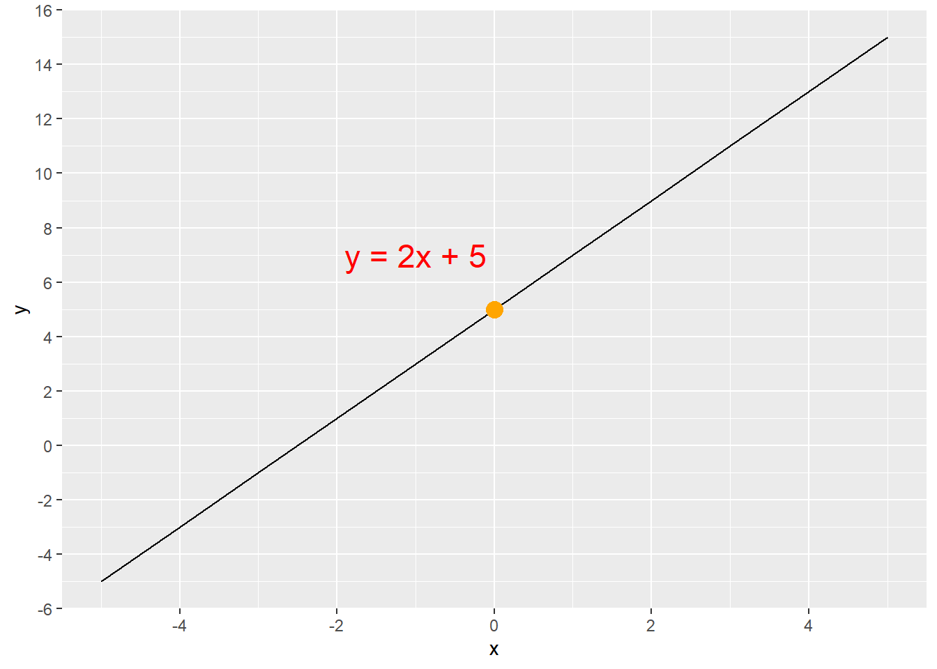
The equation y = 2x + 5 produces the line shown in Figure 5.1. The y-intercept is at (0,5), which is the orange dot. We can find any value of y for any given value of x by simply multiplying x by 2 and then adding 5. If x = 4, then y = 13, because (2 * 4) + 5 = 13. Thus, the line goes through the point (4,13). This can be confirmed in Figure 5.1.

There is a positive linear relationship between the value of x and the value of y in the equation y= 2x + 5 because m > 0. As x increases, y also increases.

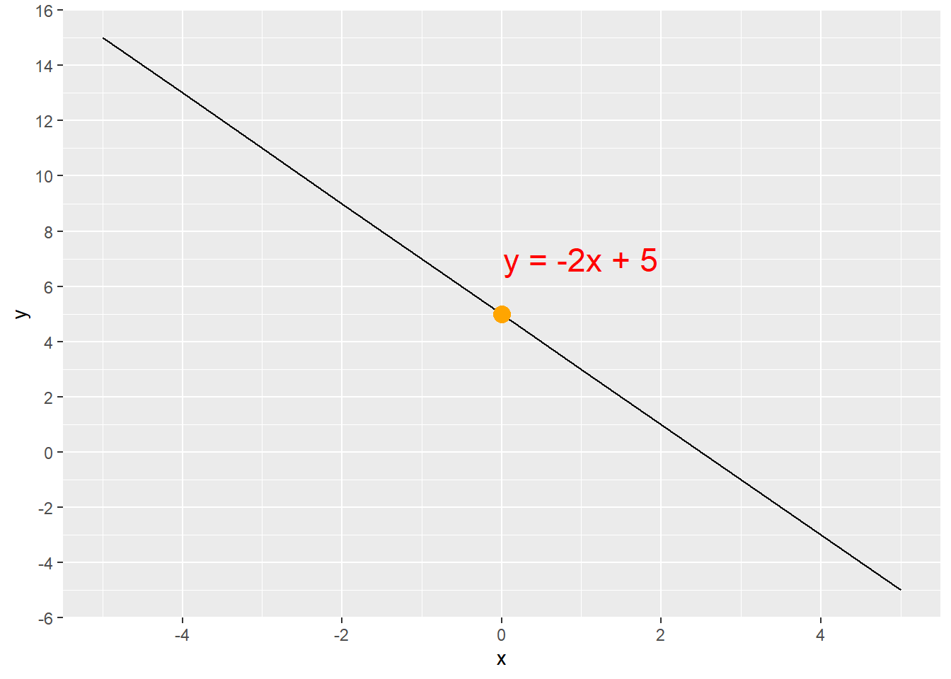
Figure 5.1: Slope-intercept equation of a line (positive linear relationship between x and y)

Notice what changing the coefficient m to a negative number does to the line (Figure 5.2). There is a negative linear relationship between the value of x and the value of y in the equation y= -2x + 5 because m < 0. As x increases, y decreases.

Figure 5.2: Slope-intercept equation of a line (negative linear relationship between x and y)

5.1.2 Linear regression equation

We transition from the slope-intercept equation of a line to regression by expressing the equation in different terms. Equations Equation 5.4 and Equation 5.5 are identical. The terms have simply been renamed and rearranged into the format of linear regression. We use the Greek letter β, which is the lower-case beta (B), and represent the y-intercept with β₀ and the slope with β₁. The x is represented with x₁ to clearly show that it is tied to β₁. This subscripting will become important as we add more x variables.

\[y = mx + b \tag{5.4}\]

\[y = \beta_{0} + \beta_{1}x_{1} \tag{5.5}\]

Equation 5.5 is called simple linear regression because there is only one x variable. Linear regression analysis of data most often results in multiple linear regression where there are multiple x variables as shown in Equation 5.6. This equation differentiates the x variables and corresponding coefficients (a.k.a parameters) with subscripts. Note that we no longer have a slope. Instead, we have coefficients β₁, β₂, β₃, …, β_n that are each tied to an x variable x₁, x₂, x₃, …, x_n.

\[y = \beta_{0} + \beta_{1}x_{1} + \beta_{2}x_{2} + \beta_{3}x_{3} + ... + \beta_{n}x_{n} \tag{5.6}\]

The coefficients (β₁, …, β_n ) are interpreted in the same way in both simple and multiple linear regression. Imagine a regression analysis to determine pit stop time in seconds (ps_seconds) based on crew practice hours per week (crew_hrs), average crew experience in years (crew_years), and rain in millimeters (rain_mm). This fake data (see Creating Fake Data) could return Equation 5.7, where the coefficient for crew_hrs is -0.54, the coefficient for crew_years is -1.26, and the coefficient for rain_mm is 0.78.

\[ps\_seconds = 13.78 - 0.54 * crew\_hrs - 1.26 * crew\_years + 0.78 * rain\_mm \tag{5.7}\]

ps_seconds has a negative linear relationship with crew_hrs and crew_years, which is shown by the negative coefficients. ps_seconds will decrease by 0.54 seconds for every unit increase in crew_hours if all other variables are held constant. ps_seconds will decrease by 1.26 seconds for every unit increase in crew_years if all other variables are held constant.

ps_seconds has a positive linear relationship with rain_mm, which is shown by the positive coefficient. ps_seconds will increase by 0.78 seconds for every unit increase in rain_mm if all other variables are held constant.

Linear regression equations can include binary categorical \(x\) variables (see Section 5.5.1). For binary categorical \(x\) variables, a value of \(x = 1\) causes the value of \(y\) to change by the value of the coefficient of that \(x\) variable because \(1 * β = β\). In contrast, a value of \(x = 0\) causes no change in the value of \(y\) because \(0 * β = 0\).

5.1.3 Linear regression concept

Linear regression is a mathematical process of creating a model (i.e. formula) for a line that fits a set of data points when the data points do not necessarily fall on the line.

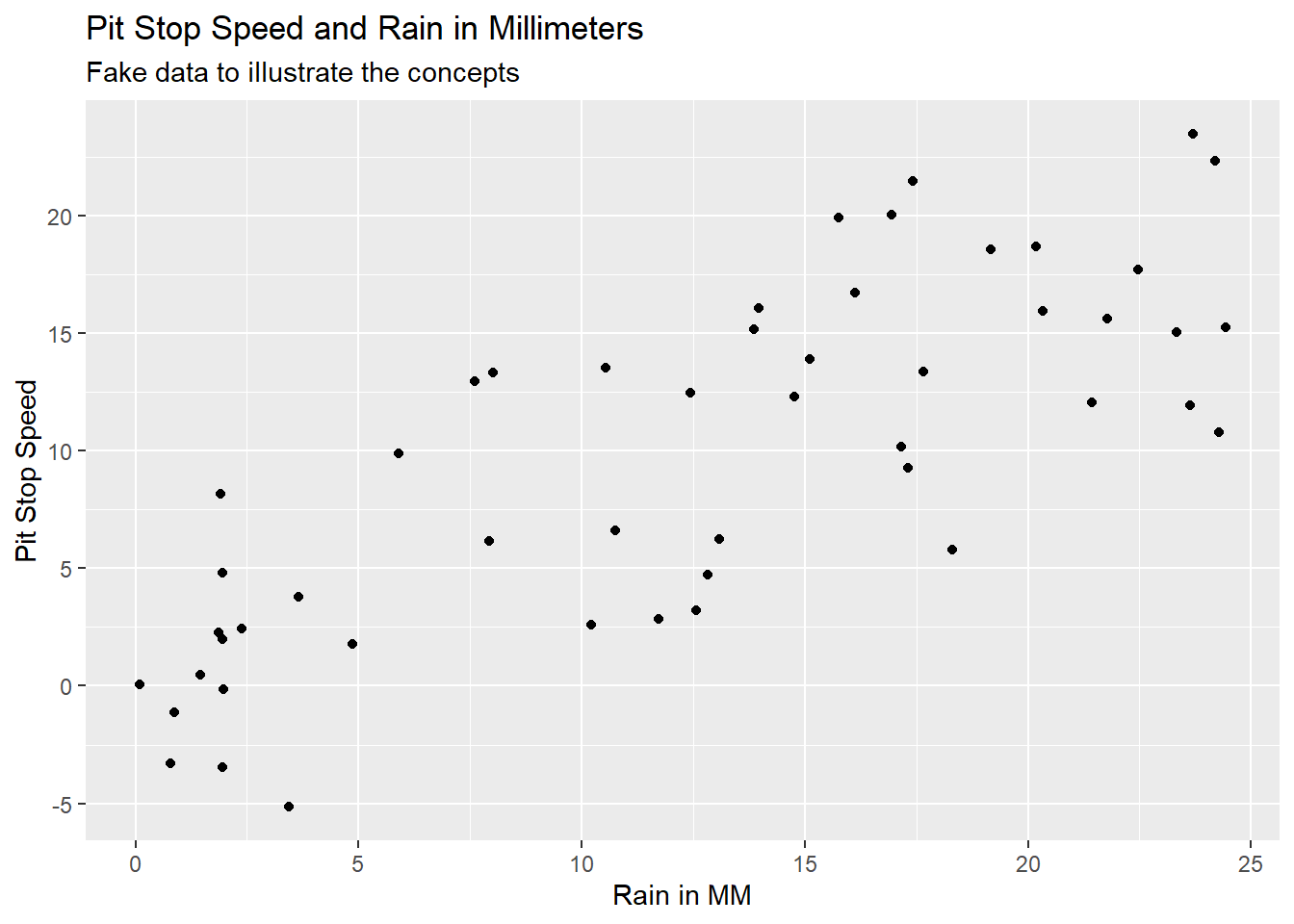
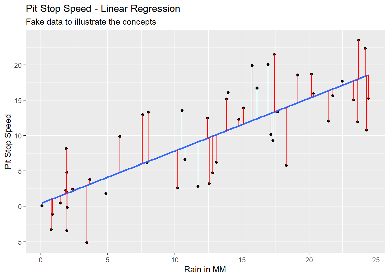
Imagine we had data on pit stop time in seconds and rain in millimeters. The data might look like Figure 5.3 with Pit Stop Speed on the y-axis and Rain in MM on the x-axis. This is fake data to illustrate the concept of linear regression.

Figure 5.3: Linear regression example with fake data

We could run a mathematical process called Ordinary Least Squares (OLS) to find the regression line of best fit through this data. Equation 5.8 would be the equation and the blue line in Figure 5.4 would be the line created with this equation.

\[ps\_seconds = 0.41 + 0.74 * rain\_mm \tag{5.8}\]

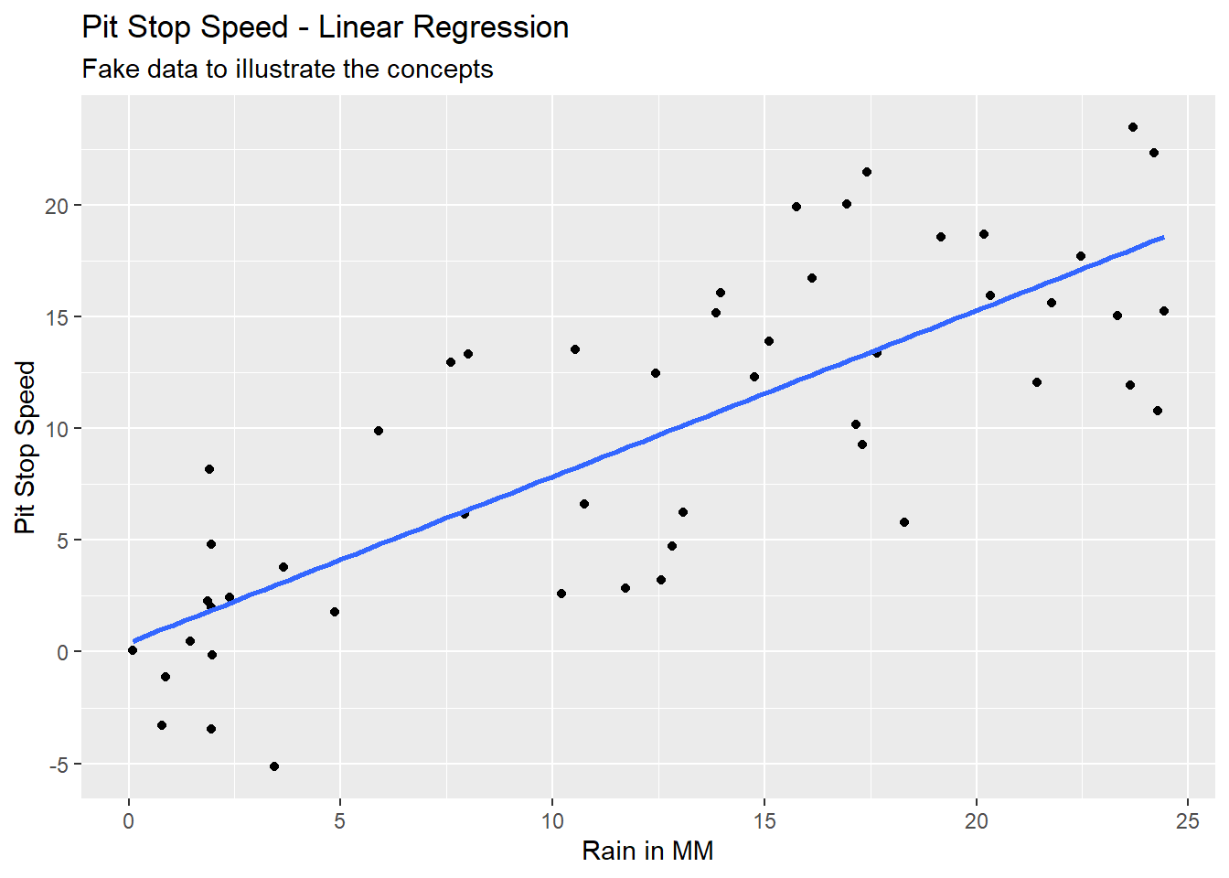
Figure 5.4: Linear regression example with fake data

Notice that the actual values of y (the black dots) in Figure 5.4 do not always fall on the line of the calculated values of y (blue line). The difference between the y actual value (y) and the y calculated value (ŷ, called y-hat) is an error term referred to as a residual. The differences are illustrated by the vertical red lines in Figure 5.5.

\[e = y - \hat{y} \tag{5.9}\]

Figure 5.5: Linear regression example with fake data

5.2 Linear Regression Assumptions

Explanations of the assumptions of linear regression are all over the board. An online search will reveal pages explaining from three to ten assumptions, often with seemingly non-overlapping complex or over-simplified explanations. The assumptions of linear regression belong to statisticians, not data analysts. I am not a statistician. I have gleaned the following assumptions from reconciling the explanations in Freund and Wilson (2003, 291–92, 319–24), Groebner, Shannon, and Fry (2014, 570–71), Jaggia et al. (2023, 261–71), Shmueli et al. (2023, 170–71), and Frost (n.d.).

I am convinced that at least part of the problem with the disparity in descriptions is the use of the word assumptions. What do we mean by assumptions? We mean requirements of the model that should be checked, and if you do not check these requirements then you are assuming they are true.

A linear regression model that violates one or more of these assumptions may still be useful for estimating \(y\) values.

Linear regression model building requirements that should be checked or assumed.

Continuous \(y\) variable: The calculated value (ŷ) from a linear regression equation is always an unbounded continuous variable. Therefore, linear regression is not suited for calculating a categorical \(y\) variable.
Linearity with \(y\): There is a linear relationship between each continuous \(x\) variable as specified and \(y\). This can be checked with bivariate scatter plots between the \(y\) variable and each \(x\) variable. The as specified refers to form of the \(x\) variables (e.g. no transformation, raised to a power, inverse, log, etc.). Anscombe (1973) quartet illustrates the need for visualizing data and the risks of using only calculated results to evaluate a data set. Anscombe’s quartet of data sets, each with \(y\) and \(x_{1}\), provides identical linear regression formulas (at two decimal places for the y-intercept and three decimals for the coefficient of \(x_{1}\)). A brief glance at Anscombe’s quartet illustrates the problem.
Low multicolinearity: Multicolilnearity refers to a linear relationship between any of the x variables {x₁, x₂, x₃, …, x_n}. We want little to no multicolinearity among our x variables because linear relationships between the x variables adversely impacts the accuracy of the coefficient calculations. Variance Inflation Factor (VIF) can be used to test for multicolinearity among the x variables. Pairwise scatter plots can be used to visually evaluate multicolinearity among the x variables.
Homoskedasticity: The residuals (i.e. the error term e calculated by Equation 5.9) have the same variance across all values of the x variables {x₁, x₂, x₃, …, x_n}. This assumption can be checked visually by looking at the spread of the residuals on a scatter plot. Qualtrics has helpful examples of residual plots.
Normally distributed residuals: The residuals (i.e. the error term e calculated by Equation 5.9) are approximately normally distributed. The quantile-quantile (Q-Q) plot can be used to evaluate this assumption. Yearsley has helpful examples of Q-Q plots.
Low correlation between residuals and each \(x\) variable: Correlation between the residuals (i.e. the error term e calculated by Equation 5.9) and any of the x variables {x₁, x₂, x₃, …, x_n} adversely impacts the accuracy of the coefficient calculations. This type of correlation is an indication of missing one or more x variables in the model (i.e. data that was excluded from the model that should have been included in the model). Residual plots (residuals against each \(x\) variable) can be used to check for this correlation.
Independent observations: The observations (i.e. rows of data) are not correlated with one another. Observations that are correlated will cause repeating patterns in the residual plot.

The following are not requirements that should be checked, but are important considerations.

Linearity in coefficients: The equation is linear in the coefficients {β₁, β₂, β₃, …, β_n}, which means no coefficient is raised to a power (other than 1) and there is no multiplication or division of a coefficient by another coefficient. This means the form of Equation 5.6 is the only possible form of coefficients for a linear regression equation. The functions used in R ensure this linearity of coefficients. This does not prevent the x variables {x₁, x₂, x₃, …, x_n} from being mathematically altered (e.g. raised to a power, inverse, log, etc.) to increase the estimation ability of the model.

5.3 Ordinary Least Squares (OLS)

Ordinary Least Squares (OLS) is the most common mathematical method used to create a linear regression model. The OLS process creates the line of best fit by minimizing the sum of squared residuals (i.e. the error term e calculated by Equation 5.9) through Equation 5.10 for each coefficients β₁ … β_n and Equation 5.11 for the y-intercept, β₀.

\[\beta_{n} = \frac{\sum (x_{i}-\bar{x}_{n})(y_{i}-\bar{y})}{\sum (x_{i}-\bar{x}_{n})^2} \tag{5.10}\]

\[\beta_{0} = \bar{y} - \beta_{1}\bar{x}_{1} - \beta_{2}\bar{x}_{2} - \beta_{3}\bar{x}_{3} - ... - \beta_{n}\bar{x}_{n} \tag{5.11}\]

The lm() function is used to run OLS regression. The first parameter of the lm() function is the variables to be used in the equation. Equation 5.12 illustrates the basic form of this parameter, which is used when there is no interaction in x variables. The ‘+’ sybmol in Equation 5.12 can be read as and. The second parameter of the lm() function is the data set to be used.

\[y \sim {x}_{1} + {x}_{2} + {x}_{3} + ... + {x}_{n} \tag{5.12}\]

# Read in the fake data
fake_data <- read_csv("fake_pitstops.csv")

# Create the linear regression model 
my_model <- lm(ps_seconds ~ crew_hrs + crew_years + rain_mm, data = fake_data)

The results of lm() should be stored in an object, my_model in this example, and can be summarized with the summary() function.

# Output the summary report of the linear regression model
summary(my_model)


Call:
lm(formula = ps_seconds ~ crew_hrs + crew_years + rain_mm, data = fake_data)

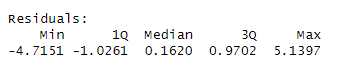
Residuals:
    Min      1Q  Median      3Q     Max 
-4.7151 -1.0261  0.1620  0.9702  5.1397 

Coefficients:
            Estimate Std. Error t value Pr(>|t|)    
(Intercept) 13.77845    1.18236   11.65 2.52e-15 ***
crew_hrs    -0.54419    0.07334   -7.42 2.15e-09 ***
crew_years  -1.26071    0.10023  -12.58  < 2e-16 ***
rain_mm      0.78215    0.04002   19.55  < 2e-16 ***
---
Signif. codes:  0 '***' 0.001 '**' 0.01 '*' 0.05 '.' 0.1 ' ' 1

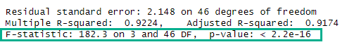
Residual standard error: 2.148 on 46 degrees of freedom
Multiple R-squared:  0.9224,    Adjusted R-squared:  0.9174 
F-statistic: 182.3 on 3 and 46 DF,  p-value: < 2.2e-16

The summary output provides the y-intercept (Figure 5.6, green box) and coefficients for the x variables (Figure 5.6, yellow box), which allows us to write the equation in Equation 5.13.

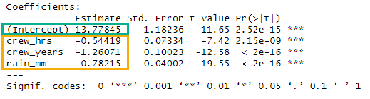
Figure 5.6: Linear Regression y-Intercept and Coefficients

\[ps\_seconds = 13.78 - 0.54 * crew\_hrs - 1.26 * crew\_years + 0.78 * rain\_mm \tag{5.13}\]

5.4 Model Performance Metrics

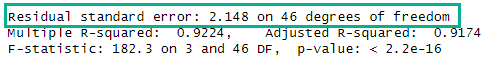
Residual Standard Error: The standard deviation of the residuals. The fake pit stop data has a residual standard error of 2.148 seconds, which means the model predicts the pit stop seconds with an average error of 2.148 seconds.

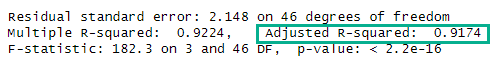
Adjusted R-Squared: The coefficient of determination, which provides the proportion of the variance in y explained by the model. The fake pit stop data has an adjusted R-squared of 0.9174. Thus, the model explains 91.74% of the variance in ps_seconds. Adjusted R-squared is used when there are multiple x variables. R-squared, strangely named Multiple R-squared in the summary() output, is used for simple linear regression (i.e. when there is only one x variable). Adjusted R-squared applies a small penalty for each additional x variable.

F-Statistic and associated p-value: The F-test provides the joint significance of a regression model via the F-statistic and p-value. If the F-test p-value is below your significance level then you can reject the model’s null hypothesis. The F-statistic must be compared to the critical value with the qf() function or online lookup tables. The model is statistically significant If the F-statistic is greater than or equal to the critical value. The linear equation (Equation 5.13) for the fake pit stop data is statistically significant because 182.3 > 2.80.

The null hypothesis for the model states that the model has no ability to explain the variance in the y variable. The p-value describes the probability of getting the results achieved if the null hypothesis is true. Statistics by Jim has a great article on statistical significance.

# Calculate the critical value for the F-statistic from the fake pit stop data.
# Using a significance level of 0.05.
qf(p = .05, df1 = 3, df2 = 46, lower.tail = FALSE)

[1] 2.806845

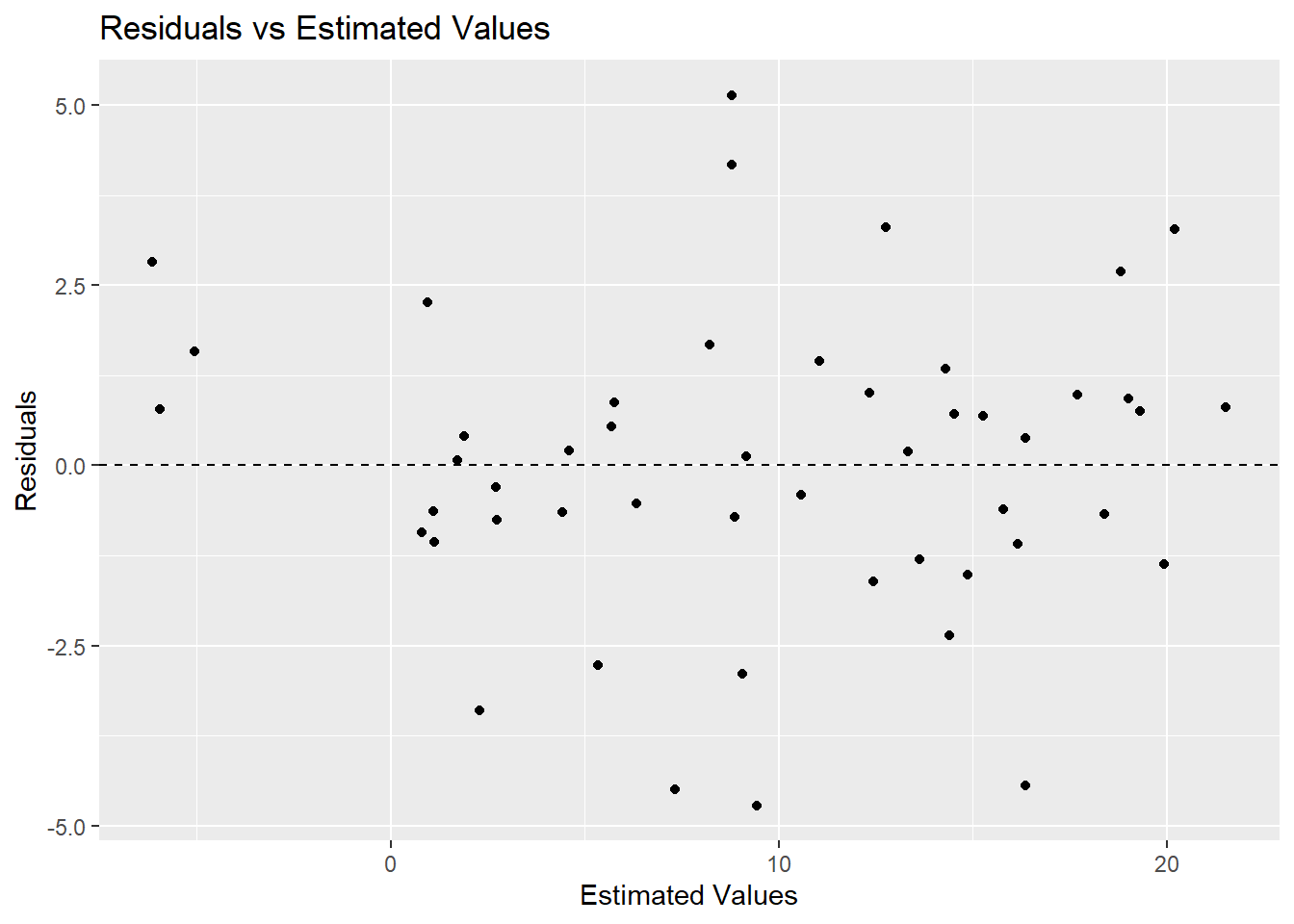
Residuals: Residuals are the difference between the actual (y ) and the estimated (ŷ ) (Equation 5.9). The summary() output provides range statistics for the residuals. Plotting the residuals can aid in evaluating the results of a model in relation to the assumptions of linear regression (Section 5.2).

ggplot(data = my_model,
       mapping = aes(x = .fitted, y = .resid)) +
  geom_point() + 
  geom_hline(yintercept = 0, linetype = 2) +
  labs(
    title = "Residuals vs Estimated Values",
    x = "Estimated Values",
    y = "Residuals"
  )

Figure 5.11: Linear regression residuals

5.5 Model Building Techniques

5.5.1 Working with categorical data

Regression requires all x variables to be numeric. So how do we handle categorical variables that are represented by words? We use one-hot encoding.

Consider a fake data set with two variables: x1 contains the categories yes and no ; x2 contains the categories warm, hot, and cold. These variables can each be converted to dummy variables through the one-hot encoding method.

One-hot encoding creates a new variable for each category in the original variable and assigns values of either 0 or 1. An illustration will help with understanding this concept.

library(fastDummies)  # Easy method for creating dummy variables via one-hot encoding

# Read in the fake data
fake_cat <- read_csv("fake_categorical.csv")

# Show the first 10 rows
head(fake_cat, 10)

# A tibble: 10 × 2
   x1    x2   
   <chr> <chr>
 1 no    hot  
 2 no    warm 
 3 yes   hot  
 4 no    warm 
 5 yes   warm 
 6 yes   hot  
 7 no    hot  
 8 yes   hot  
 9 no    warm 
10 yes   warm

# Make dummy variables
fake_cat <- dummy_cols(fake_cat)

# Alternatively, the ifelse() function can be used, but it is tedious
# fake_cat$x1_no <- ifelse(df$x1 == "no", 1, 0)
# fake_cat$x1_yes <- ifelse(df$x1 == "yes", 1, 0)

# Show the first 10 rows
head(fake_cat, 10)

# A tibble: 10 × 7
   x1    x2    x1_no x1_yes x2_cold x2_hot x2_warm
   <chr> <chr> <int>  <int>   <int>  <int>   <int>
 1 no    hot       1      0       0      1       0
 2 no    warm      1      0       0      0       1
 3 yes   hot       0      1       0      1       0
 4 no    warm      1      0       0      0       1
 5 yes   warm      0      1       0      0       1
 6 yes   hot       0      1       0      1       0
 7 no    hot       1      0       0      1       0
 8 yes   hot       0      1       0      1       0
 9 no    warm      1      0       0      0       1
10 yes   warm      0      1       0      0       1

Notice in the output above that new variables have been created for each category in x1 and for each category in x2. Also notice that for any given category the 1 in the dummy variable indicates the category was selected in the original variable, and the 0 in the dummy variable indicates the category was not selected in the original variable. For example, when a specific row of x1 contains no, then the same row of x1_no contains a 1 and the same row of x1_yes contains a 0.

——-The k-1 rule in regression is very important!——-

k-1 rule: Use one less dummy variable in building a regression model than there are categories in the original categorical variable.

The x1 variable has two categories: yes and no. Thus, we must use one dummy variable in regression model building. Choose either x1_yes or x1_no, but not both. It makes little difference which one we select.

The x2 variable has three categories: warm, hot, and cold. Thus, we must use two dummy variables in regression model building. Choose any combination of two dummy variables, such as x2_hot and x2_cold, but not all three. It makes little difference which two we select.

The k-1 rule avoids perfect multicolinearity (Section 5.2). This is based on the concept of degrees of freedom. There are k-1 degrees of freedom in a categorical variable.

If x1_yes = 0 then x1_no must equal 1. If x1_yes = 1 then x1_no must equal 0.

If x2_hot = 0 and x2_cold = 0 then x2_warm must equal 1. If x2_hot = 1 or x2_cold = 1 then *x2_warm must equal 0.

5.5.2 P-values of individual coefficients

The illustration of OLS in Section 5.3 is idealized. All the calculations worked out perfectly because the data was created for this purpose. Real data creates real problems for OLS, which must be addressed.

Consider the following model, which is based on adding the average crew age (crew_age) to the model used in Section 5.3. This is fake data (see Creating Fake Data), which, again, has been designed to illustrate a concept.

# Create the linear regression model 
model4 <- lm(ps_seconds ~ crew_hrs + crew_years + rain_mm + crew_age, data = fake_data)
summary(model4)


Call:
lm(formula = ps_seconds ~ crew_hrs + crew_years + rain_mm + crew_age, 
    data = fake_data)

Residuals:
    Min      1Q  Median      3Q     Max 
-4.6437 -0.9409  0.1268  1.0339  4.9482 

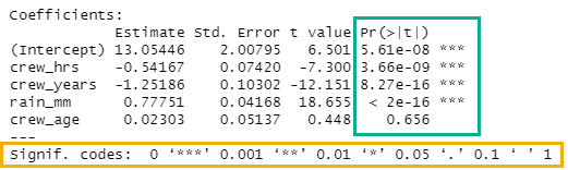
Coefficients:
            Estimate Std. Error t value Pr(>|t|)    
(Intercept) 13.05446    2.00795   6.501 5.61e-08 ***
crew_hrs    -0.54167    0.07420  -7.300 3.66e-09 ***
crew_years  -1.25186    0.10302 -12.151 8.27e-16 ***
rain_mm      0.77751    0.04168  18.655  < 2e-16 ***
crew_age     0.02303    0.05137   0.448    0.656    
---
Signif. codes:  0 '***' 0.001 '**' 0.01 '*' 0.05 '.' 0.1 ' ' 1

Residual standard error: 2.167 on 45 degrees of freedom
Multiple R-squared:  0.9228,    Adjusted R-squared:  0.9159 
F-statistic: 134.4 on 4 and 45 DF,  p-value: < 2.2e-16

If the p-value of an individual coefficient (Figure 5.12) is below the chosen significance level then the null hypothesis can be rejected for that specific x variable. The p-value is listed as a number (green box under Pr(>|t|)) and scored with an asterisk system, which allows quick comparison to standard significant levels (yellow box). If we choose a significance level of 0.05, then the p-value for crew_age is too high. Thus we cannot reject the null hypothesis for this variable at the 0.05 significance level. Therefore, crew_age must be removed from our model to create a valid model. Always remove individual x variables one at a time starting with the x variable with the highest p-value. Remove one x varaible, then rerun the OLS. Repeat until all x variables have a p-value less than the chosen significance level.

The null hypothesis for each x variable states that the variable has no impact on the y variable. The p-value describes the probability of getting the results achieved if the null hypothesis is true. Statistics by Jim has a great article on statistical significance.

5.5.3 Stepwise

5.5.4 Recursive feature elimination (RFE)

5.6 Model Application

The predict() function is used to apply a model to a data set. The result of the following code is one value, thus the 1 in the output, and an estimate of 17.52 seconds. This is the exact, or fitted, estimate given the data and the model.

#Estimate the value of *y* based on the model and specified data
predict(my_model, data.frame(crew_hrs = 2.5, crew_years = 3.4, rain_mm = 12))

       1 
17.51739

The following code creates an estimate for every observation in the data set.

#Estimate the value of *y* based on the model and the data already associated with the model
#Add the estimate as a new variable to the data frame.
fake_data$estimate <- predict(my_model)